DRAFT OF 8/25/08
An Evaluation of the Scale Invariant Feature Transform (SIFT)
Theo Pavlidis ©2008
Abstract
An approximate analysis of SIFT combined with numerical results on the properties of extrema on which SIFT is based is used to suggest certain limitations of the transform. A set of images was selected to test this hypothesis and actual tests with an implementation of SIFT confirmed the limitations. SIFT appears to be useful in CBIR only when searching for nearly identical images. This is the case in forensic applications and in intellectual property disputes but it is hard to think of other applications.
1. Introduction
The Scale Invariant Feature Transform (SIFT) has been proposed by D. Lowe [Lo04] as a tool for Content Based Image Retrieval (CBIR) and it has been used for that purpose by some authors (for example, [SZ08] and [LJJ08]). It has also been found lacking in some applications [Ba07].
SIFT is based on convolving an image with a Gaussian kernel for several values of the variance σ and then taking the difference between adjacent convolved images. If D(x, y, σ) denotes such differences, then the method is based on finding extrema of this function with respect to all the three variables. Such maxima are candidates for keypoints that, after additional analysis, are used to characterize objects in an image.
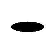
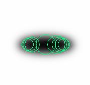
Extrema of D(x, y, σ) with respect to all the variables, i.e. candidates for keypoints (CK) occur when the support of the Gaussian kernel matches (at least approximately) the shape of the (gray scale) image function. Such a "tuning" property in the scale space has been known so one may argue that SIFT acts as a local frequency transform. However such extrema may occur in other positions as well. [Lo04] discusses this issue briefly in Section 3.1 without any analysis. The paper states that for a circle the maximum occurs at the center when the "circular positive central region of the difference-of-Gaussian function matches the size and location of the circle. For a very elongated ellipse, there will be two maxima near each end of the ellipse." It seems that the actual situation is more complex. In order to reduce the clutter on images I consider only maxima of D(x, y, σ) and figures that are black on a white background. Figure F1 shows the original shape (A), all the maxima found (B), and the two strongest maxima (C).
 |
 |
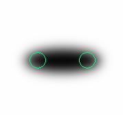 |
| A. An Ellipse | B. Maxima found denoted by circles centered at the maximum and with radius proportional to σ | C. Only the strongest maxima are shown. (Measured by the difference from the next value.) |
Figure F1 |
||
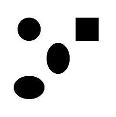
Extrema seem to occur not only as a result of matching a shape with the support of a kernel but also in other points in response to local curvature. This is also illustrated in Figure F2.
 |
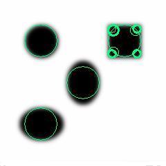 |
| A. Four geometrical shapes | B. Maxima found denoted by circles centered at the maximum and with radius proportional to σ. Note the multitude of extra maxima in the case of the square. |
Figure F2 |
|
While [Lo04] suggests several ways to select keypoints from the candidate keypoints, there is no precise characterization of keypoints in terms of human perception of an image. Furthermore, the experience with the results of implementations of SIFT supports the view that there is no well defined connection between keypoints and the perceptual characteristics of an image. It is possible to obtain some analytical results for a limited class of images, as shown next.
2. The Case of Separable Images
In order to simplify the analysis I consider a separable image, one where
the gray scale function I(x,y) can be expressed
as the product of two functions: I(x,y) = X(x)Y(y).
The Gaussian kernel is also separable,
g(x, y, σ) = h(x, σ)h(y, σ) so
that the convolution of a separable image with a Gaussian kernel can be
expressed as the product of two one-dimensional convolutions, XC(x,
σ) and YC(y, σ). If
two successive values of σ have ratio q,
(q>1), then we have
| D(x, y, σ) = XC(x, σ)YC(y, σ) - XC(x, qσ)YC(y, qσ) | (E1) |
| Dx(x, y, σ) = XCx(x, σ)YC(y, σ) - XCx(x, qσ)YC(y, qσ) | (E2) |
| Dx(x, y, σ) = h(x, σ)YC(y, σ) - h(x, qσ)YC(y, qσ) | (E3a) |
| Dy(x, y, σ) = h(y, σ)XC(x, σ) - h(y, qσ)XC(x, qσ) | (E3b) |
YC(y, qσ) over YC(y, σ) is bounded by q and a similar property holds for XC(), then there will be values of x (or y) that satisfy both equations as illustrated in Figure F3. Because of the symmetric from of Eqs. (E3a) and (E3b) zeros will occur when x and y are the same so that they will be along the diagonal of the corner.
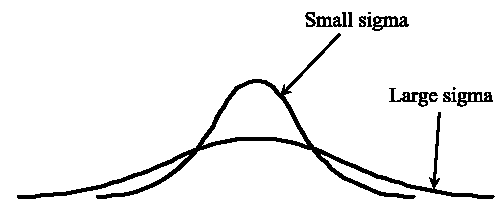 |
Figure F3: Illustration of how Gaussian kernels always intersect. The same is true for any kernel that has a constant integral value. |
Therefore we may expect several locations of extrema in x and y and the only issue is to find extrema with respect to σ. Appendices A and B show specific examples. Because we cannot solve the Gaussian case analytically, the analysis is performed for the case of a "boxcar" kernel with support S and constant amplitude 1/S (so its area is one) and it is followed by numerical results for the Gaussian case. We consider two cases. In the first the one dimensional function is a pulse so that the image contains a right rectangle (Appendix A). In the second the one dimensional function is a step, so that the image contains a corner with a vertical and a horizontal side (Appendix B).
The results confirm that candidates for keypoints occur not only when the support of the Gaussian kernel matches a shape, but also at several other points as predicted from Equ. (E3).
3. A Controlled Test of SIFT to Illustrate the Consequences of the Nature of the Keypoints
In order to illustrate the above observations I selected a set of images with careful control of their characteristics. Professor Anil Jain of Michigan State University kindly agreed to have one of his doctoral students, Ms. Jung-Eun Lee, run a SIFT matching implementation on the images I submitted. I should point out that I sent only one set of images which included the images I had posted as a Challenge to CBIR. I have presented all the results either here or in my note on Meeting Some of the Challenges. Thus I had committed myself to the images before seeing the results of SIFT.
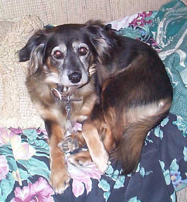
Figure F4 shows the seven images used in the tests. The captions include the dimension of the image, the number of keypoints found by the SIFT method, and, in parentheses, the average number of pixels per keypoint..

|
|

|
A: 191X123 kpts = 320 (73) |
B: 191X123 kpts = 323 (73) |
F: 721X480 kpts = 9770 (35) |
|
 |
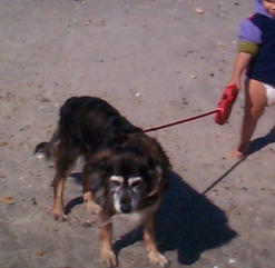 |
G: 609X658 kpts = 7875 (51) |
H: 455X286 kpts = 2219 (59) |
J: 247X241 kpts = 565 (105) |
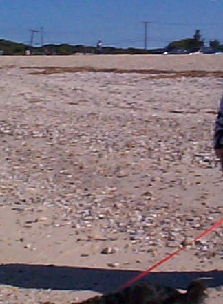 |
Figure F4: Images used in the tests. Images A and F have been cropped from a larger image in slightly different locations. In addition, A was subsampled by a factor of 4 in each dimension. B was derived from A by a brightness increase transformation. The captions include the dimension of the image, the number of keypoints found by the SIFT method, and, in parentheses, the average number of pixels per keypoint. Click on an image to see it in full size. Each image will be displayed in a separate window, so that they can be compared visually in detail. |
|
K: 324X442 kpts = 2762 (52) |
||
The table below shows the results of the matching by SIFT keypoints in pairs of images from Figure F4.
| Image Pair | Number of Keypoints Matched | Display of matched Keypoints |
|---|---|---|
| A and B | 205 | Click here |
| A and F | 405 | Click here |
| A and G | 235 | Click here |
| A and H | 59 | See Figure F5 below. |
| A and J | 7 | See Figure F6 below. |
| J and K | 91 | See Figure F7 below. |
Because of the brightness scale invariance of SIFT one would expected many matching key points for the pair A, B and this is indeed what happened as shown in the first row of the table. For this pair of images the performance of SIFT is far superior than that of algorithms based on color histograms or edge histograms. (The brightness enhancement transformation distorts both histograms in a significant way while the semantics remain unaltered.) For images A and F the performance of SIFT continues to be good, as expected. Because of the difference in pose of the main object, there only half as many matching keypoints in the A, G pair as they were in the A, F pair. Does such a drop agree with human impressions? Clearly, SIFT very well in matching images that are nearly identical, but even relatively small changes produce a big drop in matching points.
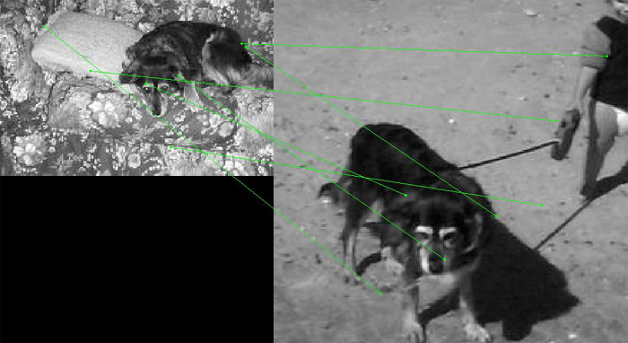
The A, H pair presents a bigger challenge because H includes the subject of A in a different pose and with other object present. Figure F5 shows the matching of the keypoints.
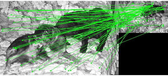 |
Figure F5: Matching of key
points on images A and H |
Finally, SIFT does poorly in the pair A, J as expected because the object common in the two images is in significantly different poses. Figure F6 shows the matching of the keypoints.
|
Figure F6: Matching of key
points on images A and J. (Click on the image to see it full size.) |
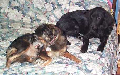
I also thought to be interesting to compare image J and one centered on the beach ground (K). That produced several matches as shown in the Table and in Figure F7 below.
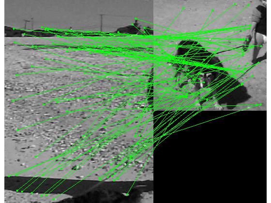 |
Figure F7: Matching of key
points on images J and K |
There are many keypoint matches not only between parts of the ground but also between parts if the dog and the ground. Note that image J appears to be more similar to K (91 matches) than to A (7 matches) which is not the answer that one looking for pictures of the dog would have liked. On the other hand, if one looks at images as a whole, then J and K are certainly more similar to each other than the A, J pair.
4. Conclusions
Both the approximate analysis and the numerical simulations confirm that extrema do occur at points where the support of the kernel matches roughly the area of a shape (Figure F.B) but also in other places that have no connection with image features. Keypoints depend strongly on local properties of a representation of an object and cannot be expected to capture properties of solid objects. They depend on the properties of the projection of on object, not on the properties of the object itself. This was confirmed with the tests of Section 3, in particular Figure F6. Therefore they can be useful in matching image of 3D objects that have the same pose or images of 2D objects. In either case it is important that the object of interest occupies most of the area of the images, otherwise spurious matchings may occur.
A major characteristic of keypoints is that the luminance of the image does not enter in their definition. This can be both advantage (as in the case of matching images A and B in Section 3) but it can also be a disadvantage because slight variations in luminance will produce candidates for keypoints similar to those produced by large variations.
One consequence of the close connection between the support of the kernel and the size of variations in a image is that blurring will produce major changes in the candidates for keypoints. If we assume that the blurring kernel is also Gaussian with variance σ1 then convolving the blurred image with a Gaussian with variance σ2 will be the same as convolving the original image with Gaussian kernel with variance σ , where σ is given by
| σ = sqrt ( (σ1)2 + (σ2)2) | (E4) |
Because of the lack of perceptual significance of the keypoints, SIFT can be used to match images that are supposed to be nearly identical (as A, B, and F are), but not just similar (as A and G or H are). This is not a problem in the forensic application discussed in [LJJ08] where a tattoo image must be matched with an identical one in a database (if such an entry exists). Another potential application of SIFT is in intellectual property searches where one looks for nearly identical images. (The case of images A, B, and F offers such an example, all three have been produced from the same original.)
The big question (given the computational cost of SIFT) is whether there are simpler ways to achieve the same result.
5. Works Cited
[Ba07] T. Bakken "An Evaluation of the SIFT algorithm for CBIR"
Telnor R&I Research Note N30/2007.
Source on the web.
[Lo04] D. Lowe "Distinctive Image Features from scale-invariant keypoints" Int. J. Comp. Vision, 2004.
[LJJ08] J-E. Lee, A. K. Jain, R. Jin "Scars, Marks, and Tattoos (SMT): Soft Biometric for Suspect and Victim Identification" Biometrics Symposium, Tampa, Sept. 2008.
[SZ08] J. Sivic and A. Zisserman "Efficient Visual Search for Objects in Videos", IEEE Proceedings, Special Issue on Multimedia Information Retrieval, 96 (4), 2008, pp. 548-566.
[We] Weisstein, Eric W. "Convolution." From MathWorld--A
Wolfram Web Resource. http://mathworld.wolfram.com/Convolution.html