A Set of Images for Testing CBIR Techniques and a Collection of Results
© Copyright 2008, 2009 by T. Pavlidis
Contents
2.1. Results using local histogram modality
2.2. Results using SIFT keypoints (courtesy A. K. Jain and Jung-Eun Lee, Michigan State University)
Abstract: I supply a set of images that present challenges of different degree to CBIR methods. Satisfying Equ. (1) should be easy for any modern method. Satisfying Eqs. (2) and (3) is a more difficult task that current methods do not seem to be able to handle. In the results sections there are examples of two methods that satisfy Equ. (1) but not the other two.
1. The Images
This is a set of images, most of them containing a dog, that I have used in the past to evaluate CBIR techniques. Matching the picture of a dog poses a harder challenge than matching the pictures of solid objects because a dog can have a large variety of poses. I posted some of the images as part of a "Challenge to CBIR" about a year ago and I am creating this new document as a result of discussions I had during the ICPR08 in December 2008.
A CBIR method that makes any claim to generality should be able to calculate a measure of similarity (or distance) between any pair of images because in a general system any image can be a query and any image can be a member of the database. Even a special purpose CBIR system should be able to evaluate the similarity between any pair of images and some examples of such systems are shown in Section 2.
The key characteristic of the set is that images have degrees of similarities from each other and that allows the careful evaluation of CBIR methods. It is possible to create similar sets for other objects and such a larger collection would offer a better test set but even this small set can provide interesting insights.
The set of eleven images is shown at the end of this Section.
Images A and F have been cropped from a larger image in slightly different locations. In addition, A was subsampled by a factor of 4 in each dimension. Image B was derived from A by a brightness increase transformation. Image G is of similar size to F and only in a slightly different pose. Therefore a CBIR method that is invariant with respect to illumination and geometric scales should find A, B, and F nearly identical and G only slightly different.
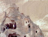
Image C is a landscape from Cappadocia and it was chosen because it has similar color histograms to B. I came across the example by looking for the pictures most similar to B (on the basis of color histograms) from my personal collection and C was the closest. The triplet of images A, B, and C can serve as a challenge to CBIR methods based on global histograms. Such methods would find that B is much more like C than A, in direct contrast to the semantic interpretation. I posted these three images in January of 2008 with that claim and no one has attempted to prove me wrong.
If Sim(I, J) denotes the similarity of a pair of images I and J, any credible CBIR method must find
| Sim(A,B) >> Sim(A, C) and Sim(A,B) >> Sim(B,C) | (1a) |
If Dist(I, J) denotes the distance between a pair of images I and J, any credible CBIR method must find
| Dist(A,B) << Dist(A, C) and Dist(A,B) << Dist(B,C) | (1b) |
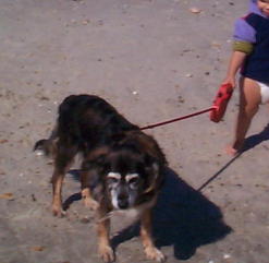
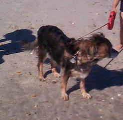
Image H is a picture of two dogs presenting a greater challenge to a query while images D and E are pictures of the same dog as in image A but in a different pose and with a different background. Finally image K is an image of the background of images D and E. Semantically we should have
| Sim(A, D) >> Sim(D, K) | (2a) |
| Dist(A, D) << Dist(D, K) | (2b) |
However satisfying such conditions seems quite hard under the current state of the art.
Images L and M present the greatest challenge. According to [1] "A striking characteristic of the human visual recognition process is its ability to overcome obstructions in the retinal image ... so that recognition remains largely unaffected by such obstructions". [1] goes on to present experiments using vertical bars. Since human viewers are not bothered by the bars we should expect
| Sim(G, L) >> Sim(L, M) or Dist(G, L) << Dist(L, M) | (3) |
If a CIBR method achieves that feat, it will be very impressive.
|
|
|
|
A (real size) |
B (real size) |
C (real size) |


|
|
D [J] (real size) |
E (real size) |

|

|
F (click to see full size image) |
G (click to see full size image) |
 |
 |
H (click to see full size image) |
K (click to see full size image) |
 |
 |
L (real size) | M
(real size) |
2. Results by various methods
2.1. Results on the test set using local histogram modality
In this method each image is converted to luminance (gray) values and it is divided into dxd squares. On each square the local luminance histogram is classified as being single peak over a narrow zone ("flat" region), bimodal with distinct peaks ("sharp" region), or of none of the above forms ("full" region). The modality of the histograms is calculated by using adaptive multi-thresholding. The percentage of such regions on an image is counted and the resulting three numbers are used as a feature vector. Because we deal with percentage the method is relatively insensitive to the image size. Also because we deal with histogram modalities it is relatively insensitive to illumination. The method fails when d is comparable to the image dimensions because the histograms are no longer local. Because the method is so simple and uses only three features, it is not a serious contender for CBIR. It is included here in order to show how the tests should be conducted.
The following tables show some results for the above set using this simple method. (Distances have been rounded to the nearest integer.)
|
|
||||||||||||||||||||||||||||||||||||||||||||||||||||||||||||||||||||||||||||||||||||||||||||||||||
Image A is used as query in Table 1 and the shortest list displays image according to their similarity to A. d equaled 8 and the Linf norm was used for the comparisons. This image metric assigns B, F, and H as been the closest to A in agreement with human intuition. However, it fails after that, although one may find some consolation that M was judged the most distant image. It satisfies the first part of Equ. (1b) but it fails with Equ. (2b).
Table 2 lists the 20 most similar pairs for d equal to 16 and the L2 norm. Pairs that may be considered close by a human observer are marked in green. The results satisfy Equ. (1b): Dist(A, B) is 13 (No. 8 in the table) and that is less than Dist(A, C) that is 31 and Dist(B, C) that is 22. (The latter are No. 39 and No. 21 respectively in the table of all pairwise distances.) However they fail both Equ. (2b) and Equ. (3).
Click here for results for other values of d and other norms as well as for a complete list of all 55 pairwise distances.
Clearly, the method performs poorly as a general image similarity measure although in some cases, it provides results in agreement with human intuition. Table 1 presents a more positive view of the method than Table 2 and one reason that the tables are included here is to show that one cannot judge a method by its success in selected cases only.
There was no "training" or any adjustments of the method to the test figures.
2.2. Results on the test set using SIFT keypoints [2]
These tests were carried out by Ms. Jung-Eun Lee, a doctoral student at Michigan State University working under the supervision of Professor Anil Jain. The percentage is calculated from the ratio of matches to the the number of keypoints in the smaller of the two images. It is possible to have one keypoint in a small image match several in a large image, so the ratio may exceed 100%.
| Image Pair | Number of matching SIFT keypoints | Percent |
|---|---|---|
| A, B | 205 |
64% |
| A, C | 4 |
|
| B, C | 2 |
|
| D, E | 108 |
|
| A, E | 10 |
|
| C, E | 4 |
|
| A, D | 7 |
about 2% |
| A, F | 405 |
127% |
| A, G | 235 |
73% |
| A, H | 59 |
18% |
| D, K | 91 |
16% |
| Large numbers denote proximity | ||
Matching SIFT keypoints clearly provides more reliable results than local histograms. For example: (i) The similarity between A and G is greater than that between A and H which is in agreement with human intuition, while local histograms list H as more similar to A than G to A. (ii) The similarity between C and E is very low while Table 2 shows a short distance between them. The method satisfies Equ. (1a) in a stronger way than the method of Section 2.1 satisfies Equ. (1b). However it fails to satisfy Equ. (2a).
There was no "training" or any adjustments of the method to the test figure.
3. Cited Works
1. Y. Lerner, T. Hendler, and R. Malach "Object-completion Effects in the Human Lateral Occipital Complex", Cerebral Cortex, 12 (2002), pp. 163-177.
2. D. Lowe "Distinctive Image Features from scale-invariant keypoints" Int. J. Comp. Vision, 2004.